Boundary State

Tree DP

A local choice fixes the boundary, then child subtrees become independent DP pieces.

postorderMISFPT

01Rootorient tree

02Takeblock child

03Skipmerge child

04Bagtreewidth k

take/skip2 states

bag choices2^k

compatibilityoverlap

DP Problem on Trees

Maximize Independent Set on Trees 最大独立集

Input: an undirected tree $G=(V,E)$.

Output: an independent set with maximum cardinality, namely the largest possible number of selected vertices.

Independent Set: a set $S\subseteq V$ such that no two selected vertices are adjacent:

$$\mathrm{\forall }u,v\in S,(u,v)\notin E$$

最大独立集在一般图上是 NP-hard 的；但是当图是一棵树时，结构足够简单，可以用 DP 或者等价的 greedy idea 在线性时间解决。

Recursive View

Root the tree at an arbitrary vertex $r$.

对于某个节点 $v$，考虑它的 subtree rooted at $v$。我们有两个选择：

1. Choose $v$.
2. Do not choose $v$.

如果选择 $v$，那么它的所有 children 都不能被选；下一层可以重新自由选择，所以问题会落到 grandchildren 的子树上。

如果不选择 $v$，那么它的 children 可以自由决定是否选择，所以问题会落到 children 的子树上。

Subproblem Definition

先定义一个单状态 DP：

$$f[v]=\text{maximum size of independent set in the subtree rooted at }v$$

Then:

$$f[v]=max\{\sum _{u\in children(v)}f[u],1+\sum _{g\in grandchildren(v)}f[g]\}$$

含义：

• 第一项：不选 $v$，所以每个 child 的 subtree 都可以取最优。
• 第二项：选 $v$，拿到 $1$，但是不能选 children，只能从 grandchildren 的 subtree 继续取最优。

The topological order is bottom-up, usually postorder traversal.

A Cleaner Two-State DP

实际写代码时，更常用 two-state DP：

$$take[v]=1+\sum _{u\in children(v)}skip[u]$$$$skip[v]=\sum _{u\in children(v)}max\{take[u],skip[u]\}$$

Answer:

$$max\{take[r],skip[r]\}$$

这里：

• $take[v]$: max independent set size in subtree $v$ when $v$ is selected.
• $skip[v]$: max independent set size in subtree $v$ when $v$ is not selected.

This avoids explicitly iterating over grandchildren, but it is the same idea.

Complexity

每个 vertex 只会被处理一次，每条 parent-child 关系也只参与常数次转移。

$$Time=O(|V|)$$$$Space=O(|V|)$$

Greedy View on Trees

这个 tree DP 也可以从 greedy 的角度理解。

Greedy idea:

1. Choose all current leaves.
2. Remove all leaves' parents.
3. Repeat on the remaining forest.

为什么可以这样做？

If a leaf $\ell$ has parent $p$, then choosing $\ell$ only conflicts with $p$. If a solution chooses $p$, we can often replace $p$ by its leaf children without making the solution smaller. So there exists an optimal solution containing the current leaves.

The process is equivalent to solving the DP bottom-up:

• leaves are selected,
• their parents become blocked,
• then the remaining graph decomposes into smaller trees.

Implementation can be $O(|V|)$ by maintaining degrees and a queue of current leaves.

queue = all leaves
while queue is not empty:
    take all current leaves into answer
    mark their parents as removed
    update degrees of the remaining neighbors
    newly created leaves enter queue

This greedy formulation is useful for intuition, while the DP formulation is safer to generalize.

Independent Set on General Graphs

一般图不像树，因为 cycle 和 clique 会让“父子子树独立”这个结构消失。

但是有些图看起来 almost like a tree。如果我们把一个小的 dense part, such as a triangle, 看成一个 super node，图可能重新变成 tree-like。

For a super node with $k$ vertices:

• there are at most $2^k$ ways to choose vertices inside it;
• each way creates different restrictions for adjacent super nodes;
• we can design a DP state like $f[i,way]$.

If the largest super node has size $k$, many problems can be solved in:

$$O(2^{O(k)}\cdot n)$$

This motivates treewidth.

Treewidth Idea

Treewidth measures how close a graph is to a tree.

Informally:

• 把图拆成一棵 tree of bags；
• each bag contains several original vertices;
• smaller bags mean the graph is more tree-like.

If the largest bag has size $k+1$, then:

$$treewidth=k$$

Examples:

• Tree: treewidth $1$.
• Cycle: treewidth $2$.
• Clique on $n$ vertices: treewidth $n-1$.
• Series-parallel graphs: treewidth at most $2$.

Many optimization problems become:

$$O(2^{O(k)}\cdot poly(n))$$

when parameterized by treewidth $k$.

This is called Fixed-Parameter Tractable, or FPT:

$$O(f(k)\cdot n^c)$$

Here $f(k)$ can be exponential, but the exponent of $n$ is constant.

Tree Decomposition

A tree decomposition is a tree whose nodes are bags of vertices.

Let $B(t)$ be the bag at tree node $t$.

Requirements:

1. Every graph vertex appears in at least one bag.
2. For every graph edge $(u,v)$, there is a bag containing both $u$ and $v$.
3. For every graph vertex $x$, all bags containing $x$ form a connected subtree.

The treewidth of this decomposition is:

$$\underset{t}{max}|B(t)|-1$$

The treewidth of the graph is the minimum value over all possible decompositions.

Separation Property

Root the tree decomposition.

For a decomposition node $u$, its bag $B(u)$ separates different child subtrees.

Intuition:

• vertices inside one child subtree can interact with the parent side only through $B(u)$;
• two different child subtrees are independent once $B(u)$ is fixed.

This is exactly why DP works: once we decide which vertices in the boundary bag are selected, each child subtree can be solved independently.

Notation:

• $B(u)$: bag at decomposition node $u$.
• $T(u)$: subtree of the decomposition rooted at $u$.
• $B(T(u))$: union of all bags inside $T(u)$.

DP on Tree Decomposition for MIS

Goal: solve Maximum Independent Set on a graph with treewidth $k$.

Root the tree decomposition.

Define:

$$f[S,u]$$

as the maximum size of an independent set $I\subseteq B(T(u))$, under the condition:

$$I\cap B(u)=S$$

where:

$$S\subseteq B(u)$$

If $S$ itself is not an independent set, then:

$$f[S,u]=-\mathrm{\infty }$$

Base Case

If $u$ is a leaf in the tree decomposition:

$$f[S,u]=|S|$$

if $S$ is independent; otherwise:

$$f[S,u]=-\mathrm{\infty }$$

Transition

Suppose $a$ is a child of $u$ in the tree decomposition.

The parent state fixes $S\subseteq B(u)$. For child $a$, we need to choose a child bag state:

$$S^{\prime }\subseteq B(a)$$

that is compatible with $S$ on the overlap:

$$S^{\prime }\cap B(u)=S\cap B(a)$$

Then the best contribution from child $a$ is:

$$\underset{\begin{array}{c}{S}^{\prime }\subseteq B(a)\\ S^{\prime }\cap B(u)=S\cap B(a)\end{array}}{max}(f[S^{\prime },a]-|S\cap B(a)|)$$

The subtraction avoids double counting the vertices in the overlap between parent and child bags.

Therefore:

$$f[S,u]=|S|+\sum _{a\in children(u)}\underset{\begin{array}{c}{S}^{\prime }\subseteq B(a)\\ S^{\prime }\cap B(u)=S\cap B(a)\end{array}}{max}(f[S^{\prime },a]-|S\cap B(a)|)$$

The final answer at root $r$ is:

$$\underset{S\subseteq B(r)}{max}f[S,r]$$

Complexity

If treewidth is $k$, then every bag has at most $k+1$ vertices.

Number of states per bag:

$$2^{k+1}$$

For each parent state, checking compatible child states can cost another factor $2^{k+1}$. So the charged transition cost is:

$$O(4^k)$$

Total running time, given a tree decomposition:

$$O(4^{k}n)$$

The important takeaway:

Tree DP works not only on trees, but also on graphs that can be decomposed into small bags arranged as a tree.

Network Flow

在多项式时间内精确求解问题的算法，不断迭代求解

问题描述

以轨道运输为例，对一个有向图$G(V,E)$, 每条边上有 Edge capacity，用来表述该边最多可以承载多少passenger。

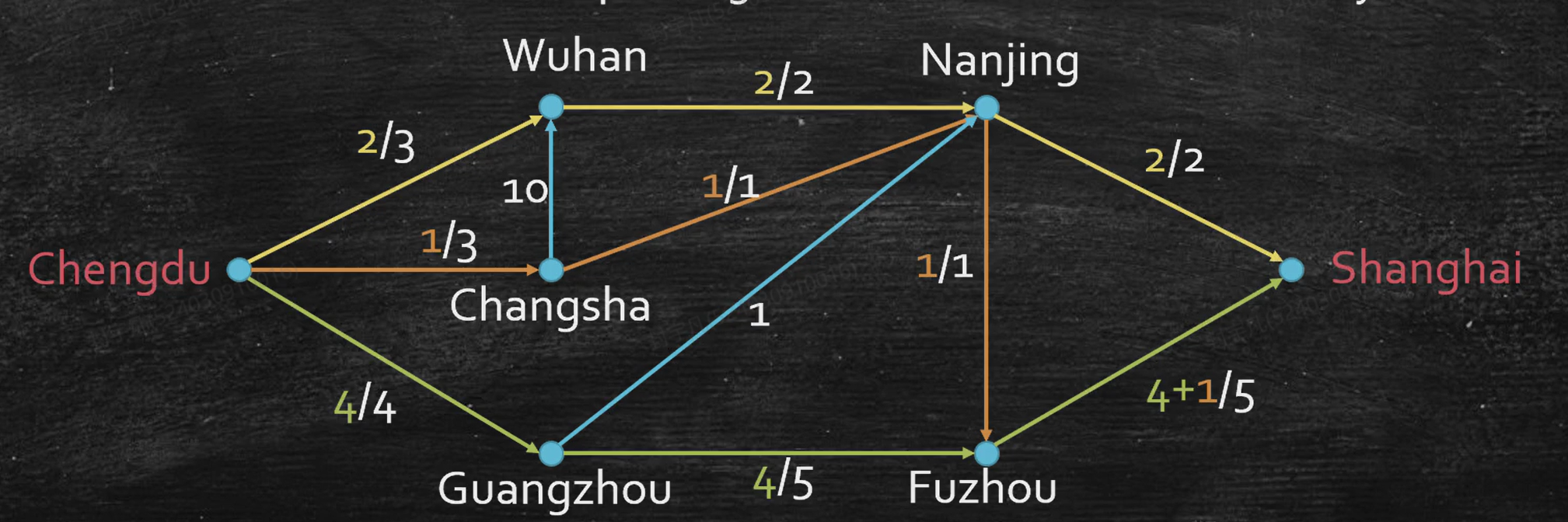
问题的formalize

Given a directed graph $G=(V,E)$, source $s\in V$, sink $t\in V$, and capacity function

$$c:E\to {\mathbb{R}}_{\ge 0}$$

a Flow is a function

$$f:E\to {\mathbb{R}}_{\ge 0}$$

where $f(e)$ means the amount of flow sent through edge $e$.

For $f$ to be a feasible flow, it must satisfy:

Capacity Constraint

For each edge $e\in E$,

$$0\le f(e)\le c(e)$$

Flow Conservation

For each vertex $u\in V\setminus \{s,t\}$, the total incoming flow equals the total outgoing flow:

$$\sum _{v:(v,u)\in E}f(v,u)=\sum _{w:(u,w)\in E}f(u,w)$$

Total Flow

The value of a flow is the total flow leaving the source:

$$v(f)=\sum _{v:(s,v)\in E}f(s,v)$$

Equivalently, for any feasible flow,

$$v(f)=\sum _{u:(u,t)\in E}f(u,t)$$

So the Maximum Flow Problem is:

$$\underset{f}{max}v(f)$$

subject to the capacity constraint and flow conservation.

Ford-Fulkerson Algorithm

一个自然的 greedy idea 是：

不断找一条从 $s$ 到 $t$ 的路径，然后沿着这条路径尽可能多地 push flow。

但是这个做法如果只在原图 $G$ 上找路径，会遇到问题：前面选错的路径可能占用了某些边的容量，导致后面无法继续增广。
所以我们需要允许算法 cancel 一部分已经送出去的 flow，也就是在残量网络里加入 backward edge。

Residual Network

Given a feasible flow $f$, the residual network $G_f=(V,E_f)$ describes how we can still adjust the current flow.

For each original edge $(u,v)\in E$:

• If $f(u,v)<c(u,v)$, add a forward residual edge $(u,v)$ with residual capacity

$$c_f(u,v)=c(u,v)-f(u,v)$$

• If $f(u,v)>0$, add a backward residual edge $(v,u)$ with residual capacity

$$c_f(v,u)=f(u,v)$$

Intuition:

• forward edge means we can send more flow on the original edge;
• backward edge means we can cancel part of the flow already sent on the original edge.

Augmenting Path

An augmenting path is an $s$-$t$ path $P$ in the residual network $G_f$.

The amount of flow we can push through $P$ is limited by the bottleneck residual capacity:

$$b=\underset{e\in P}{min}{c}_f(e)$$

Then for every residual edge on $P$:

• if it is a forward edge $(u,v)$, update

$$f(u,v)\leftarrow f(u,v)+b$$

• if it is a backward edge $(v,u)$ corresponding to original edge $(u,v)$, update

$$f(u,v)\leftarrow f(u,v)-b$$

Algorithm

FordFulkerson(G=(V,E), s, t, c):
    initialize f(e) = 0 for every e in E
    construct the residual network G_f

    while there exists an s-t path P in G_f:
        b = min residual capacity of edges on P

        for each residual edge e on P:
            if e is a forward edge (u,v):
                f(u,v) = f(u,v) + b
            if e is a backward edge (v,u) for original edge (u,v):
                f(u,v) = f(u,v) - b

        update G_f

    return f

The algorithm stops when there is no $s$-$t$ path in $G_f$. At this point, no more flow can be pushed from $s$ to $t$.

Small Bug: Anti-parallel Edges

If the original graph contains both $(u,v)$ and $(v,u)$, then a residual edge direction alone is not enough to distinguish:

• a real forward edge;
• a backward edge used to cancel flow.

One standard fix is to transform the graph so that no anti-parallel edges exist, or explicitly tag each residual edge as forward/backward.

Termination

If all capacities are integers, then each augmentation increases $v(f)$ by at least $1$. Therefore Ford-Fulkerson halts in at most $f_{max}$ iterations.

With a DFS/BFS search for each augmenting path, one iteration costs $O(|E|)$, so for integer capacities:

$$O(|E|\cdot f_{max})$$

For rational capacities, we can rescale them into integers. For irrational capacities, Ford-Fulkerson may not halt depending on how augmenting paths are chosen.